
Backprop in Neural Networks
Published:
This article serves as a good exercise to see how forward propagation works and then how the gradients are computed to implement the backpropagation algorithm. Also, the reader will get comfortable with the computation of vector, tensor derivatives and vector/matrix calculus. A useful document can be found here for the interested reader to get familiar with tensor operations.
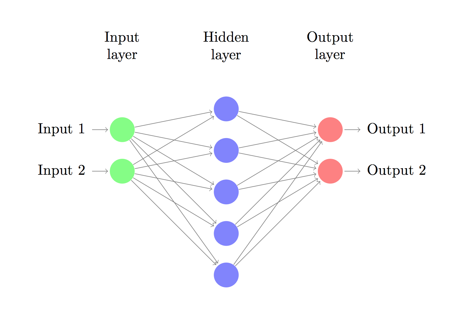
We will compute the gradients and derivatives of the loss function of the given neural network as shown in the Fig 1. with respect to the parameters: \(W_{1}\), \(W_{2}\), \(b_{1}\) and \(b_{2}\). Where \(W_{1}\), \(W_{2}\) are the weight matrices; and \(b_{1}\) and \(b_{2}\) are bias the vectors. Let \(x \in \mathcal{R}^2\), \(W_{1} \in \mathcal{R}^{2*500}\), \(b_{1} \in \mathcal{R}^{500}\), \(W_{2} \in \mathcal{R}^{500*2}\) and \(b_{2} \in \mathcal{R}^2\). Also, show how the forward and backpropagation algorithms work.
Let us first compute the forward propagation. Let x be the input. The first hidden layer is computed as follows: \[z_{1} = \textit{x}W_{1} + b_{1} \tag{1}\]
We then apply a non-linear activation function to equation \[a_{1} = \textit{tanh}(z_{1}) \tag{2}\]
The output layers’ activation are obtained using the following transformation \[z_{2} = a_{1}W_{2} + b_{2} \tag{3}\]
Finally, a softmax is applied to get:
\[a_{2} = \hat{y} = softmax(z_{2}) \tag{4}\]
where \(\hat{y}\) is the predicted output by the feedforward network
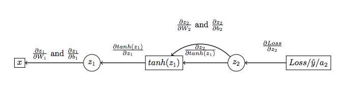
Let’s see this feedforward network through a circuit diagram as illustrated in Fig 2. Now, let’s see how the derivatives are computed with respect to the hidden nodes and bias vectors. Refer Fig 3.

We have to compute the derivative of the loss function with respect to \(W_{1}\), \(W_{2}\), \(b_{1}\) and \(b_{2}\) that is see the effect of these parameters on the loss function (which we actually have to minimize).
Below are the steps to compute the various gradients as shown in figure:
\[Loss = y * ln(\sigma(z_{2})) + (1-y) * ln(1-\sigma(z_{2})) \tag{5}\]
Also, note that:
\[\frac{d\sigma(z_{2})}{dz} = ln(\sigma(z_{2})) * ln(1-\sigma(z_{2})) \tag{6}\]
Therefore, \[\frac{\partial Loss}{\partial z_{2}} = y - \sigma(z_{2}) = y - \hat{y} \tag{7}\]
Since, \(\sigma(z_{2})\) = \(\hat{y}\)
\[\frac{\partial z_{2}}{\partial w_{2}} = \frac{\partial (a_{1}W_{2}+b_{2})}{\partial w_{2}} = a_{1} \tag{8}\]
\[\frac{\partial z_{2}}{\partial b_{2}} = 1 \tag{9}\]
\[\begin{aligned} \frac{\partial z_{2}}{\partial tanh(z_{1})} &= \frac{\partial(a_{1}W_{2}+b_{2})} {\partial tanh(z_{1})}\\ &= \frac{\partial(tanh(z_{1})W_{2}+b_{2})} {\partial tanh(z_{1})}\\ &= z_{2} \end{aligned}\tag{10}\]
\[\frac{\partial tanh(z_{1})}{\partial z_{1}} = 1 - tanh^2(z_{1}) \tag{11}\]
\[\frac{\partial z_{1}}{\partial W_{1}} = \frac{\partial (xW_{1}+b_{1})}{\partial W_{1}} = x \tag{12}\]
\[\frac{\partial z_{1}}{\partial b_{1}} = \frac{\partial (xW_{1}+b_{1})}{\partial b_{1}} = 1 \tag{13}\]
Finally, we can now use the chain rule to compute the effect of the four parameters namely \(W_{1}\), \(W_{2}\), \(b_{1}\) and \(b_{2}\) on the Loss function.
In what follows, \((P)^T\) indicates the transpose of some matrix or vector P.
\[\frac{\partial Loss}{\partial W_{2}} = \frac{\partial Loss}{\partial z_{2}} * \frac{\partial z_{2}}{\partial W_{2}} = a_{1}^T(y-\hat{y}) \tag{14}\]
\[\frac{\partial Loss}{\partial b_{2}} = \frac{\partial Loss}{\partial z_{2}} * \frac{\partial z_{2}}{\partial b_{2}} = (y-\hat{y}) \tag{15}\]
\[\begin{aligned} \frac{\partial Loss}{\partial W_{1}} &= \frac{\partial Loss}{\partial z_{2}} * \frac{\partial z_{2}}{\partial z_{1}} * \frac{\partial z_{1}}{\partial W_{1}} \\ &= \frac{\partial Loss}{\partial z_{2}} * \frac{\partial z_{2} }{\partial tanh(z_{1})} * \frac{\partial tanh(z_{1})}{\partial z_{1}} * \frac{\partial z_{1}}{\partial W_{1}} \\ &= x^T (1-tanh^2Z_{1}) (y-\hat{y}) W_{2}^T \end{aligned}\tag{16}\]
\[\begin{aligned} \frac{\partial Loss}{\partial b_{1}} &= \frac{\partial Loss}{\partial z_{2}} * \frac{\partial z_{2}}{\partial z_{1}} * \frac{\partial z_{1}}{\partial W_{1}} \\ &= \frac{\partial Loss}{\partial z_{2}} * \frac{\partial z_{2} }{\partial tanh(z_{1})} * \frac{\partial tanh(z_{1})}{\partial z_{1}} * \frac{\partial z_{1}}{\partial b_{1}}\\ &= (1-tanh^2Z_{1}) (y-\hat{y}) W_{2}^T \end{aligned}\tag{17}\]
Hence, we have computed both the forward propagation and back propagation for the given multi-layer neural network.